![By Wpcpey [CC BY-SA 4.0 (https://creativecommons.org/licenses/by-sa/4.0)], from Wikimedia Commons](https://www.michaelplazzer.com/wp-content/uploads/2018/11/Bourke_Street_Mall_night_view_2017.jpg)
Building a machine learning model to predict a number is a trivial exercise with today’s tools. With highly optimised models, improving the accuracy of the prediction will always be dependent on the data, and clever ways of using it. This will be the subject of this article, we’ll use R and machine learning to predict pedestrian numbers in Melbourne.
We’ll step through this in two parts:
- adding new data to your existing data set.
- feature engineering – using the data that you have to make new variables
The data
The Melbourne city council provides a cool tool to explore the data here http://www.pedestrian.melbourne.vic.gov.au. We can download it directly into R:
library(dplyr)
# this takes a minute
ped_data <- read.csv("https://data.melbourne.vic.gov.au/api/views/b2ak-trbp/rows.csv?accessType=DOWNLOAD") |
It is updated monthly, it looks like the following:
| ID | Date_Time | Year | Month | Mdate | Day | Time | Sensor_ID | Sensor_Name | Hourly_Counts |
|---|---|---|---|---|---|---|---|---|---|
| 2286872 | 2018-07-01T10:00:00 | 2018 | July | 1 | Sunday | 10 | 39 | Alfred Place | 160 |
| 2286991 | 2018-07-01T13:00:00 | 2018 | July | 1 | Sunday | 13 | 4 | Town Hall (West) | 2852 |
| 2286992 | 2018-07-01T13:00:00 | 2018 | July | 1 | Sunday | 13 | 5 | Princes Bridge | 3350 |
| 2287071 | 2018-07-01T14:00:00 | 2018 | July | 1 | Sunday | 14 | 37 | Lygon St (East) | 278 |
| 2287072 | 2018-07-01T14:00:00 | 2018 | July | 1 | Sunday | 14 | 39 | Alfred Place | 94 |
| 2287191 | 2018-07-01T17:00:00 | 2018 | July | 1 | Sunday | 17 | 4 | Town Hall (West) | 2332 |
Let’s look at just one location, Bourke Street Mall (South) in Melbourne’s CBD. We can visualise this using the ggplot2 library.
library(ggplot2) library(lubridate) ped_data %>% filter(Sensor_Name == "Bourke Street Mall (South)") %>% mutate(Date_Time = ymd_hms(Date_Time)) %>% ggplot(aes(y = Hourly_Counts, x = Date_Time)) + geom_line(aes(group = Sensor_Name, colour = Sensor_Name)) + theme(legend.position="bottom") + ylim(2000, 7500) |
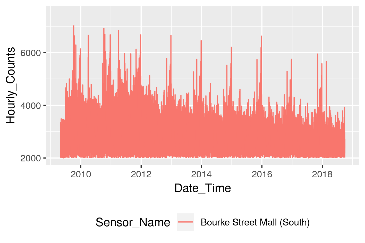
Interestingly, we can see a slow but steady long term decline in overall numbers, despite Melbourn’e population increasing in those years. There are strong peaks around Christmas/New Years, and secondary peaks that possibly represent school holidays. Using just this data, we can build our predictive model.
Basic Feature Engineering
This is a fancy way of saying “add a column”. Let’s extract the basic time information from the Date_Time field:
- month
- day of month
- time of day
model_data <- ped_data %>%
  filter(Sensor_Name == "Bourke Street Mall (South)") %>%
  transmute(Date_Time = ymd_hms(Date_Time),
            Month = lubridate::month(Date_Time),
            Day = mday(Date_Time),
            Time = lubridate::hour(Date_Time),
            Hourly_Counts) %>%
  filter(lubridate::year(Date_Time) > 2014) %>%
mutate(Date_Time = as.factor(Date_Time)) |
Let’s take a look. This is the basic structure of the input to train a model to predict Hourly_Counts:
| Date_Time | Month | Day | Time | Hourly_Counts |
|---|---|---|---|---|
| 2015-01-01 00:00:00 | 1 | 1 | 0 | 867 |
| 2015-01-01 01:00:00 | 1 | 1 | 1 | 614 |
| 2015-01-01 02:00:00 | 1 | 1 | 2 | 397 |
| 2015-01-01 03:00:00 | 1 | 1 | 3 | 239 |
| 2015-01-01 04:00:00 | 1 | 1 | 4 | 111 |
| 2015-01-01 05:00:00 | 1 | 1 | 5 | 52 |
Basic Machine Learning model
We can use the h2o framework to carry out our machine learning. To set it up we split the data into:
- training data set to build our model
- test set to measure accuracy of the model
library("h2o")
h2o.init()
h2o_model_data1 <- as.h2o(model_data)

h2o_model_data1 <- h2o.splitFrame(h2o_model_data1, 0.7) |
Our training frame is hex_h2o_model_data[[1]], and our test data will be hex_h2o_model_data[[2]]
Let’s try the extreme gradient boosting algorithm XGBoost, it seems to be winning the Kaggle competitions last time I checked. I find these algorithms are highly optimised with the default parameters. Feel free to play around with these if you feel otherwise.
training_model1 <- h2o.xgboost(training_frame = h2o_model_data1[[1]], x = -1, y = 5) |
To explain the above snippet, the fourth column is Hourly_Counts i.e. the value we’re trying to predict, so it is the ‘y’ argument in h2o parlance.
Now we use our test data set as input into the model we just built.
h2o_predicted1 <- h2o.predict(training_model1, h2o_model_data1[[2]]) test_results1 <- as.data.frame(h2o.cbind( h2o_model_data1[[2]], h2o_predicted1)) |
Let’s take a look:
| predict | Date_Time | Month | Day | Time | Hourly_Counts |
|---|---|---|---|---|---|
| 553 | 2015-01-01 01:00:00 | 1 | 1 | 1 | 614 |
| 58 | 2015-01-01 06:00:00 | 1 | 1 | 6 | 43 |
| 315 | 2015-01-01 09:00:00 | 1 | 1 | 9 | 322 |
| 833 | 2015-01-01 10:00:00 | 1 | 1 | 10 | 774 |
| 1797 | 2015-01-01 12:00:00 | 1 | 1 | 12 | 1879 |
| 2215 | 2015-01-01 13:00:00 | 1 | 1 | 13 | 2277 |
Note: Your results may vary slightly due to the stochastic nature of the algorithm.
This looks pretty good, the actual data in the Hourly_Counts column seem to track well with the data in our predict column. We can use the r2 metric to measure how well the model describes the data. An r2 equal to 1 means the model is perfect, an r2 equal to 0.5 means the model is no better than a guess.
h2o.r2(h2o.performance(training_model1, h2o_model_data1[[2]])) |
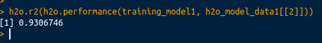
This is a great result.
Add new data
Let’s see if we can improve the r2 value by adding public holiday data. There is an excellent data source here that covers the date range we are interested in.
library(readr)
pub_hols <- read_csv("https://www.michaelplazzer.com/wp-content/uploads/2018/09/Aus_public_hols_2009-2019.csv")

# melbourne is in the state of Victoria (VIC), and we'll assign a public holiday label to those dates
pub_hols_data <- pub_hols %>%
  filter(State == "VIC") %>%
mutate(Public_Holiday = 1) |
Let’s take a look, the Day_In_Lieu field represents those days when a public holiday fell on a weekend, and the holiday was shifted to the following weekday.
| Date | State | Weekday | Day_In_Lieu | Part_Day_From | Public_Holiday |
|---|---|---|---|---|---|
| 2009-01-01 | VIC | Thursday | 0 | 0 | 1 |
| 2009-01-26 | VIC | Monday | 0 | 0 | 1 |
| 2009-03-09 | VIC | Monday | 0 | 0 | 1 |
| 2009-04-10 | VIC | Friday | 0 | 0 | 1 |
| 2009-04-11 | VIC | Saturday | 0 | 0 | 1 |
| 2009-04-12 | VIC | Sunday | 0 | 0 | 1 |
And we’ll need to join this data set with our pedestrian data, we can use the date field.
model_data2 <- model_data %>%
  mutate(Date = as.Date(Date_Time)) %>%
  left_join(pub_hols_data, by =  "Date") %>%
  select(-State, -Weekday, -Date, -Part_Day_From) %>%
  mutate(Day_In_Lieu = ifelse(is.na(Day_In_Lieu), 0, Day_In_Lieu),
         Public_Holiday = ifelse(is.na(Public_Holiday), 0, Public_Holiday)) %>%
  mutate(Day_In_Lieu = as.factor(Day_In_Lieu),
         Public_Holiday = as.factor(Public_Holiday)) %>% # be careful with factor variables
mutate(Date_Time = as.factor(Date_Time)) # h2o doesn't recognise these date types |
Let’s see what our data looks like now:
| Date_Time | Month | Day | Time | Hourly_Counts | Day_In_Lieu | Public_Holiday |
|---|---|---|---|---|---|---|
| 2015-01-01 00:00:00 | 1 | 1 | 0 | 867 | 0 | 1 |
| 2015-01-01 01:00:00 | 1 | 1 | 1 | 614 | 0 | 1 |
| 2015-01-01 02:00:00 | 1 | 1 | 2 | 397 | 0 | 1 |
| 2015-01-01 03:00:00 | 1 | 1 | 3 | 239 | 0 | 1 |
| 2015-01-01 04:00:00 | 1 | 1 | 4 | 111 | 0 | 1 |
| 2015-01-01 05:00:00 | 1 | 1 | 5 | 52 | 0 | 1 |
Now build and test the model as before.
h2o_model_data2 <- as.h2o(model_data2) h2o_model_data2 <- h2o.splitFrame(h2o_model_data2, 0.7) training_model2 <- h2o.xgboost(training_frame = h2o_model_data2[[1]], x = -1, y = 5, ignore_const_cols = FALSE ) h2o.r2(h2o.performance(training_model2 , h2o_model_data2[[2]])) |
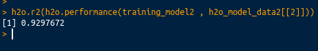
I thought that would have more benefit! The result is essentially the same, so I would consider leaving this data out. Perhaps we can work with the data that we have …
Adding more features
Let’s keep it simple: Can we increase the r2 just by adding a day of week field?
library(lubridate) library(lubridate) model_data3 <- model_data %>% mutate(Day_of_week = as.factor(weekdays(ymd_hms(Date_Time)))) h2o_model_data3 <- as.h2o(model_data3) h2o_model_data3 <- h2o.splitFrame(h2o_model_data3, 0.7) training_model3 <- h2o.xgboost(training_frame = h2o_model_data3[[1]], y = 5) h2o.r2(h2o.performance(training_model3, h2o_model_data3[[2]])) |
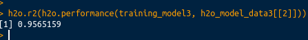
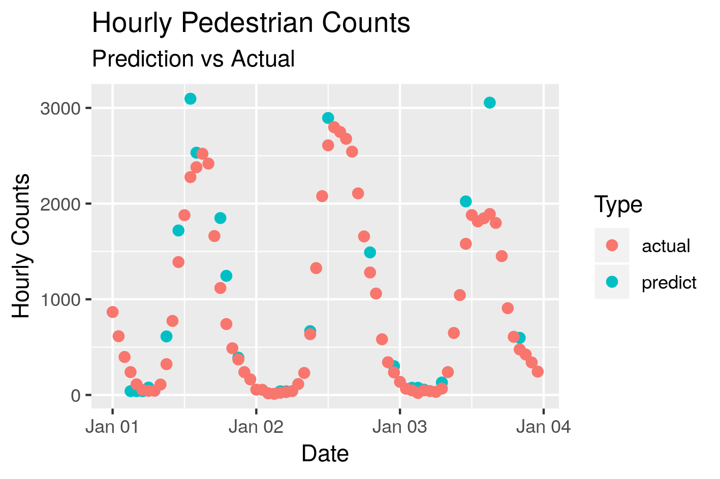
This is a substantial increase, the r2 value is getting close to one, so any new features will have diminishing returns. Let’s plot some of the predictions against the actuals
The approach described above can be applied to the other sensor locations around Melbourne. Indeed, this is a general approach that can be applied to a range of problems.